
TL;DR
We quantize Qwen3-4B from 16 to 3.60 and 2.81 bits per weight (bpw), occupying only 22% and 18% of the BF16 size, with our proprietary quantization-aware training pipeline, ORA-QAT. Training fits on a single GPU and takes about an hour on roughly 3M tokens. The checkpoints it produces can be served directly by vLLM. Both beat the standard GPTQ baseline at the same size and, remarkably, the 3-bit one retains 96.5% of full-precision quality.
Introduction
Quantization is one of the most effective levers for making large language models lighter and faster. Storing weights in fewer bits shrinks the memory footprint, reduces bandwidth pressure during decoding, and turns models that used to require a datacenter accelerator into models that run on a consumer GPU, a laptop, or an edge device. However, the price to pay is model quality degradation. The following question arises:
How far can we push quantization before the model stops being useful?
By useful we mean capable across the full range of tasks people care about, not just perplexity score in a piece of text it has never seen.
At 4 bits (e.g. INT4), the answer is fairly settled. Established post-training quantization (PTQ) methods such as GPTQ use a small calibration dataset to compensate for quantization error layer by layer, and they retain most of the quality of the full-precision BF16 baseline. In practice, 4-bit checkpoints are routinely produced for the popular models by the companies like Unsloth or RedHatAI. We take one of those checkpoints, Unsloth's bnb-4bit build of Qwen3-4B, as our reference throughout this post for what 4-bit quantization delivers.
Below 4 bits the picture changes sharply. As you move to 3, 2, or 1 bit, quality does not decay gracefully, it falls off a cliff. The degradation is strongly non-linear, and in the worst cases the model is effectively lobotomized: it stops following instructions, loses arithmetic ability, and produces text that looks fine but means nothing.
However, the resilience to quantization greatly depends on the parameter size. A large model has enough redundancy such that quantization errors can be spread thinly across many weights. A 27B model quantized to 2 bits is far more resilient than a 4B model at the same precision. That makes small models at very low precision the hardest quantization regime; and also a commercially relevant one, because small models are exactly what you want to deploy on resource constrained hardware.
This post looks exactly at this regime: a Qwen/Qwen3-4B model pushed to 3-bit and 2-bit weights.
Quality vs. size: average score against bits per weight
Average of GSM8K-Platinum, IFEval, MBPP+, MMLU-Pro and BFCL v3 for Qwen3-4B, plotted against bits per weight on a log scale. The purple line indicates a so-called Pareto frontier: the best average score reachable at a given size.
Fig. 1 — ORA-QAT holds the entire low-bit frontier. At identical bit-widths it gains 5.3 points over the GPTQ baseline at 3 bits and 27.5 points at 2 bits. Moreover, the 3-bit checkpoint retains 96% accuracy with respect to the full precision at a quarter of the disk size. Hover a point for the per-benchmark breakdown.
Using our quantization pipeline, ORA-QAT, we retain roughly 96% of full-precision quality at 3 bits and 71% at 2 bits, substantially improving on a standard GPTQ baseline at both precisions. The cost to get there is modest: about one hour of training on a single GPU and roughly 3M tokens of data. Measured against the compute typically thrown at low-bit quantization research, that is close to a free lunch. The rest of this post explains the core ideas that make it work.
Quantization-Aware Distillation
The foundation is quantization-aware training (QAT). The core mechanism is simple: during the forward pass, emulate the exact quantization scheme you intend to deploy, but keep the weights and gradient updates in full precision. The model sees the quantization error while it learns, so it can adjust its parameters to compensate for it and thus become more robust. Rather than repairing damage after the fact, the model is trained in the presence of the damage.
We take this one step further and use knowledge distillation rather than a standard language-modeling objective. The full-precision model acts as teacher, the quantized model as student, and the training signal is the Kullback-Leibler (KL) divergence between their output distributions. In our experiments this converged faster and more consistently than cross-entropy training on hard labels. The intuition is that the teacher provides a much richer target: it tells the student not just which token is correct but how the entire probability mass should be shaped, which is precisely the information that quantization tends to destroy.
Making QAT efficient without breaking deployment
QAT as it is usually formulated requires full fine-tuning of every weight, which is expensive in both time and memory. The obvious question is whether it can be combined with parameter-efficient methods such as LoRA, training only a small set of low-rank adapters instead. Turns out: it can!
However, the efficiency gained during training introduces a new problem at serving time that is easy to overlook. If you train adapters on top of a quantized base and then merge them into the weights and re-quantize the result, the final quantization no longer matches the one emulated during training.
Concretely, let us write for the quantize-dequantize step, for the base weights and for the low-rank update the adapters learn. The quantization mismatch can be written as
Training against a quantized base optimises the left-hand side, while the merged checkpoint that gets served computes the right-hand side. Since quantization is non-linear, the operations are not equivalent and the model learned to compensate for one quantization grid but is deployed on another and the benefit of training evaporates.
There are two ways out of this problem (as illustrated in the figure):
- Keep weights and adapters separate, and dequantize and merge them on the fly during inference.
- Merge them during training, and apply quantization to the fused weights, so the forward pass mimics the deployment pipeline exactly.
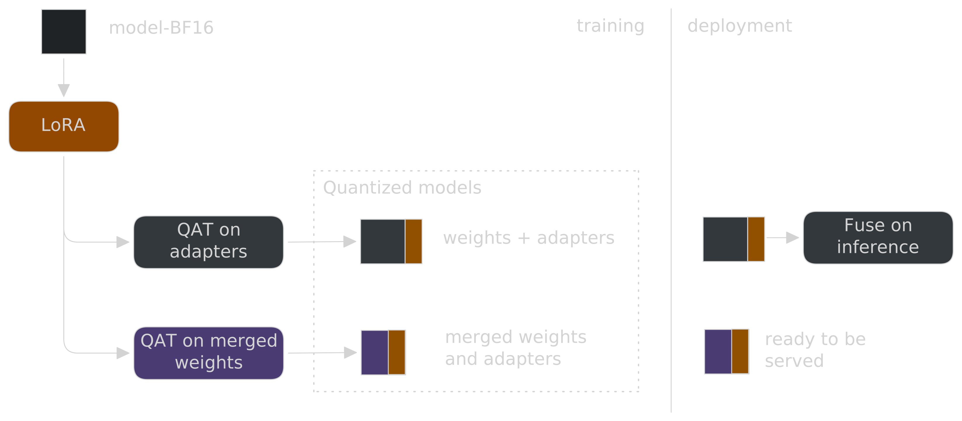
Option 1 works, but it is not hardware-friendly: it adds runtime work on every forward pass, requires an inference stack that understands the adapter structure, and carries the extra storage and complexity of shipping adapters alongside the model.
That is why we implemented Option 2. Since quantization is applied to the fused weights throughout training, the training-time forward pass and the deployment-time forward pass correspond to exactly the same computation. When training finishes, the adapters are merged with the weigths and what remains is a plain standalone quantized checkpoint which requires no custom runtime, no adapter bookkeeping, and is compatible out of the box with mainstream inference engines, also on edge devices.
Learnable quantization scales
Symmetric quantization is essentially rounding onto a regular grid. Take a group of weights and a single positive number , the scale. Each weight is stored as a small integer,
and reconstructed at inference time as . With bits, has only possible values, so the scale is what maps those few integers onto real weight magnitudes. Specifically, sets the spacing between neighbouring grid points. One scale is shared across each group of weights where each group typically contains either 64 or 128 single weights. That is why bit-width and group size are usually quoted together.
The standard choice is to derive the scale from the weights themselves, , either recomputed on every forward pass or frozen at the start of training. We instead treat the scales as learnable parameters, optimized alongside everything else. This adds an extra degree of freedom for reducing quantization loss. Frozen scales must stretch to cover the largest magnitude present, which wastes precision on the values in the center where most of the weights actually live. In turn, a learned scale can choose to clip outliers in layers where they turn out not to matter much, and spend its limited levels where they do.
Packing the model during training
Distillation needs two models in memory at the same time: the teacher in full precision and the student. For a 4B model that is roughly 8 GB each, and once activations and the rest of the training machinery are added on top, a single GPU starts to feel small. This prevents us from resource-efficient training.
Packing is what buys the room back. Rather than holding the student in full precision, we keep its weights stored in the format they will actually be deployed in, 3 or 2 bits each, and expand a layer only for the moment the forward pass needs it. The student then takes up a fraction of the space it otherwise would. Nothing about the training itself changes: updates still happen in full precision, and the model still sees the same quantization error it will meet at deployment.
For a 4B model this resource efficiency is a convenience more than a necessity. It starts to be a differentiating factor for larger models, because the saving grows with the models' size. Packing a 4B student to 3 bits frees around 6 GB; the same move on a 30B student frees closer to 45 GB during training. In this case, it is the difference between a training run that needs several GPUs and one that runs on a single GPU.
Results
We targeted two symmetric quantization schemes:
- 3-bit weights, group size 128
- 2-bit weights, group size 64
The results, against the full-precision baseline and a standard GPTQ baseline at identical bit-width and group size:
| Model | bpw | Disk | GSM8K-Platinum | IFEval | MBPP+ | MMLU-Pro | BFCL v3 | Average | Retention |
|---|---|---|---|---|---|---|---|---|---|
| Qwen3-4B BF16 | 16.0 | 7.49 GB | 90.0 | 84.9 | 71.7 | 49.2 | 84.8 | 76.1 | 100% |
| Unsloth bnb-4bit | 7.06 | 3.31 GB | 88.1 | 83.5 | 74.9 | 48.0 | 84.0 | 75.7 | 99.4% |
| GPTQ 3-bit | 3.60 | 1.68 GB | 76.7 | 79.9 | 68.0 | 40.9 | 75.5 | 68.2 | 89.6% |
| ORA-QAT 3-bit | 3.60 | 1.68 GB | 85.0 | 83.0 | 72.8 | 44.6 | 82.0 | 73.5 | 96.5% |
| GPTQ 2-bit | 2.81 | 1.31 GB | 16.0 | 49.0 | 24.1 | 16.3 | 25.8 | 26.2 | 34.5% |
| ORA-QAT 2-bit | 2.81 | 1.31 GB | 57.3 | 70.9 | 51.9 | 18.3 | 70.5 | 53.8 | 70.6% |
Two notes on the harness, for the curious: BFCL v3 covers the single-turn tasks only. Every model above was evaluated with the exact same setup, so the comparisons hold.
The bit-widths and file sizes above count the whole checkpoint, embeddings and LM head included, with both quantized to INT8 using standard llm-compressor rather than left in BF16. Qwen3-4B shares a single matrix between those two, and saving it that way is straightforward, as llm-compressor keeps it tied. Serving it is: vLLM cannot yet read the output logits off a quantized shared matrix, so the model loads without complaint and then generates gibberish. There is an open pull request adding the missing support.
Until it lands, the 3-bit checkpoint we are releasing on Hugging Face keeps both tensors in BF16, so it works with vLLM as-is, at 4.37 bpw and 2.05 GB. Internally we have a runtime that supports it, which is how we serve the INT8 variant, and it will get a post of its own soon. Moreover, quantizing the embeddings and LM head to INT8 leaves the benchmark scores practically unchanged, so the quality numbers above hold for either variant.
The benchmarks span grade-school math, instruction following, code generation, multi-domain knowledge and reasoning, and tool/function calling. Two things stand out:
At 3 bits, low-bit quantization is production-ready for this model. ORA-QAT retains 96.5% of baseline quality while occupying mere 22% of the original disk footprint, and it is ahead of the GPTQ baseline by a wide 7% margin. Coding quality is essentially unchanged; the largest remaining gaps are in math and multi-domain reasoning, the tasks that depend most on long reasoning chains of intermediate computation where small errors compound.
At 2 bits, the gain from ORA-QAT is much larger but not enough to retain decent performance. Nevertheless, the improvement over GPTQ is dramatic: the GPTQ model at 2 bits is functionally broken, with math accuracy at 16% and tool calling at 26%, while ORA-QAT recovers those to 57% and 71% respectively. This is more than double the average score at fixed bit-width! But a 29% quality loss is not acceptable for production, however impressive the relative improvement.
Size and quality can also be collapsed into a single number: how much benchmark score each gigabyte of the checkpoint actually buys. Below we consider how much quality per size each of the considered models outputs.
Quality per gigabyte
Average benchmark score divided by the size of the checkpoint on disk. Higher is better: it is the score you get back for every gigabyte you have to store and load.
Fig. 2 — Efficiency peaks at 3 bits. ORA-QAT returns more than four times as much score per gigabyte as BF16, and its 2-bit checkpoint is less efficient than its 3-bit one despite being 22% smaller.
On this axis the ordering from the table inverts. BF16 comes last by a wide margin, spreading its 76.1 points across 7.49 GB. Unsloth's bnb-4bit checkpoint, which on raw quality is essentially lossless at 99.4% retention, manages only a little over double that at 22.9 points per GB. The reason for this is honest bit counting: a nominally 4-bit checkpoint that leaves embeddings and other tensors in higher precision lands at 7.06 bpw and 3.31 GB on disk. ORA-QAT at 3 bits returns 43.6, which is 4 times more than BF16 and 1.9 times more than Unsloth. The 2.2 points of average that separate the two is what those extra 1.6 GB actually buy.
The more telling comparison is between our own two checkpoints: the 2-bit model is 22% smaller than the 3-bit one, yet lands at 40.9 against 43.6 score per GB. This means that dropping below 3 bits significantly reduces the model's quality. This is even more profound for GPTQ, which at 2 bits outputs less than half of the score per GB compared to the ORA-QAT model of identical size. In this case, the bits saved on a model are no longer useful.
Discussion
Everything above points at the same open problem: 2 bits. ORA-QAT more than doubles what GPTQ manages there, but 70.6% retention is still modest. Three directions look promising, and they are largely orthogonal.
Better codes. The scalar, uniform grid we used here is not the only option, and vector quantization with incoherence processing targets exactly this regime. QuIP# applies a randomized Hadamard transform to make the weight distribution approximately Gaussian (so-called Incoherent Processing), then quantizes weights in groups against a lattice codebook. QTIP keeps the Incoherent Processing idea but replaces the codebook with trellis-coded quantization, which reaches far higher effective dimensions at the same bitrate. Both report strong 2-bit results, and both carry the same deployment cost: a Hadamard transform inside the forward pass that not every inference stack supports, plus a non-trivial trellis decoder in QTIP's case.
Better bit allocation. The opposite approach keeps the code simple and spends the budget more carefully. The llama.cpp quantization formats, which also allow for vector quantization using I-quants, can be mixed per tensor. That is, a global bit budget can be placed where it actually buys quality instead of spread uniformly, with the result that still loads in most runtimes. We pursued that line and we'll be creating a post on this very soon!
More training. The most straightforward lever is the one we deliberately did not pull. QAT on full weight matrices instead of LoRA adapters, and with substantially more than 3M tokens, should recover considerably more quality. We kept the budget minimal on purpose: the point of this post is to demonstrate the isolated performance of QAT when it is applied to a small set of trainable parameters over a short run. Therefore, the numbers reported here represent a lower bound on what our method can achieve.
So, how far can we push quantization before the model stops being useful? For a 4B model, the line currently sits between 3 and 2 bits. At 3 bits the model holds on to nearly all of its quality out of a file less than a quarter the size. At 2 bits QAT still improves enormously on standard GPTQ, but too much quality is lost for the result to be shippable. Closing that gap will take more than what we did here: vector quantization, mixed-precision allocation, incoherence processing, or simply a much larger QAT budget.